How to get started with data wrangling

Data wrangling refers to the process used to transform raw data into a standardized, usable dataset. It’s a process most often used by data analysts and analytics engineers in order to create datasets that can be reused. In analytics engineering, data wrangling is typically done in the context of data modeling. Analytics engineers take raw data sources and manipulate them to produce data that is more readily used by the business. 

Data wrangling is important because it gives data analysts a clean dataset to work with. They don’t have to worry about renaming columns, standardizing data types, or joining datasets in the BI reporting layer. By doing this all in the wrangling process, you are ensuring data across the business meets all expectations and can be trusted. 

There are six iterative steps to the data wrangling process. You can jump to each step using the quick links below:

Data wrangling vs data cleaning

Data wrangling and data cleaning are often used interchangeably. However, data cleaning is actually only one part of the data wrangling process. While they both have similar end goals, there is much more to data wrangling. It consists of the steps taken to really understand your data and all of the nuances within it. It ensures that it contains proper business context and is ready to be used in a final business product. Data cleaning focuses on columns and their individual values and ensures they are ready to be used in grander transformations. 

If you work at a smaller scale operation such as a startup like me, then you know data wrangling starts with data discovery. Not to be confused with enterprise data discovery tools, data discovery is the process of understanding the characteristics of your data better. This is one of the key steps that differentiate it from data cleaning. The context behind the data matters! 

I like to think of data discovery as the basic SQL queries you may run when a new data source is added to your cloud data warehouse. Chances are you would want to know some simple things about your data like the number of rows, number of columns, datatypes of your columns, and how they are generated. 

In this series, we will be using the free, public Real Estate Data Atlas dataset available in the Snowflake marketplace. Feel free to download it and follow along! In this article, we will use it to highlight some key data discovery queries that you may want to run to begin your data wrangling process. 

Data discovery examples

Let’s review the main details we want to learn about a dataset when we begin the wrangling process.

Discovering the dimensions of a dataset

When I say dimensions of a dataset, I mean the length and the width. In the case of a dataset, the length is the number of rows and the width is the number of columns. You can find each of these by running some simple SQL queries

To find the row number:

SELECT COUNT(*) FROM REAL_ESTATE_DATA_ATLAS.REALESTATE.DATASETS;

You should find that there are 67 rows in this dataset, so it is fairly small.

To find the column number:

SELECT COUNT(*) FROM INFORMATION_SCHEMA.COLUMNS WHERE table_name='DATASETS';

After running this we learn that there are 13 total columns in the dataset. 

By running these simple queries you can better understand the size of the dataset you are working with. This can help you determine the types of tools you may have to use to handle the amount of data in the dataset or how long the data wrangling process will take you.

Discovering column datatypes

Knowing the datatypes of your columns is extremely important for when you begin the data cleaning phase. If you don’t have the right column datatypes, you may not be able to use the correct corresponding SQL functions. You also want to ensure these are aligned across the entire dataset. After all, standardization is a huge reason why we wrangle data in the first place!

For example, all of your date columns should be the same data datatype. All of your timestamp columns should be the same timestamp datatype (dates can be confusing!) 

Some of the most popular data types include:

• Integer

• String

• Varchar 

• Float

• Boolean

• Date

• Datetime

• Timestamp 

When previewing a dataset, you will see the names of columns and their datatypes listed. This will help you learn what types of columns you are dealing with and if you will need to cast them to other datatypes. 

If you expect one datatype and get another, it could break your entire data model because of the way a certain SQL function handles that datatype. Understand what you are working with in the beginning so you can adjust how you standardize your data across sources in the beginning of the process. 

Discovering possible problem areas

These types of queries will make up the bulk of the data discovery process. It’s important to be aware of all the potential issues with your data. Believe me, no dataset is perfect! The worst thing you can do is write transformations and not understand all of the unique edge cases that exist in your data. Awareness will help you make the right decisions with your data going forward into the data cleaning phase. 

Duplicates

Duplicates can be a huge problem when you go into the transformation phase of data wrangling. If they are present in a source dataset, they will only continue to multiply when datasets are joined together. You need to understand the granularity of your data and if it has any proper primary keys to ensure this doesn’t happen. 

Primary Keys

If you aren’t familiar with the idea of a primary key, this is essentially a column whose value is unique for every row of data. You can identify a unique row by its primary key. You should never have duplicates of this, or it is not a true primary key.

To check for primary keys:

SELECT "DatasetId" FROM REAL_ESTATE_DATA_ATLAS.REALESTATE.DATASETS GROUP BY "DatasetId" HAVING COUNT("DatasetId")>1;

Make sure you are testing the column that seems to be the primary key. I recommend looking at every _id labeled column just to be sure. Sometimes an unsuspecting column can be the true primary key of a table! 

This query should produce zero results due to the “DatasetId” column being unique. If results were returned, then you would know that there are duplicate records with that “DatasetId” column. 

NULL values

Another potential issue you should look into is the existence of NULL values. Now, NULL values aren’t always a bad thing. Sometimes they are supposed to be there! However, you want to check to see if they exist so you can understand why they exist and if they make sense in the context of your dataset. 

I recommend running the following query on every column in your dataset and documenting what you find so that you can use this in the data cleaning stage of data wrangling. 

To find NULL values:

SELECT "FirstDate" FROM REAL_ESTATE_DATA_ATLAS.REALESTATE.DATASETS WHERE "FirstDate" IS NULL;

Here you can replace the “FirstDate” column in this query with any column in the dataset in order to learn whether that column has null values or not. 

Properly handling NULL values is something we will discuss extensively in the data cleaning article of this data wrangling series. Make sure to check that out for more on dealing with NULL values! 

Moving on to data structuring 

I can’t emphasize enough how important the data discovery step is to the data wrangling process as a whole. When you don’t fully understand your data BEFORE you start the cleaning and transformation process, poor decisions are bound to happen. Make sure you look at the dimensions of your data, the datatypes of your columns, and the specific values of these columns. 

If you move forward with data cleaning without doing these things, it is likely that your datatypes will be mismatched, you won’t account for NULL values in your columns, and primary keys won’t be unique. These are all things that would lead to unreliable, low-quality data models. Don’t make these mistakes! 

Next, we will discuss the second step in data wrangling- data structuring. This is a step that depends on the specific type of data you are dealing with but is extremely helpful to know in more complex data situations.

Next, you can move on to data structuring, which is the step where you make your data usable. 

Data is often ingested into your data warehouse from various different data sources, meaning they most likely have different formats. Some of these formats include JSON objects or datasets with columns organized in a way that you can’t work with. 

For example, let’s say you have a dataset of the different flowers in your garden. One column includes all of the characteristics of each flower. Instead of listing multiple characteristics in a list within a single row in the dataset, there are multiple rows of data for each flower, each one only varying in its characteristic.

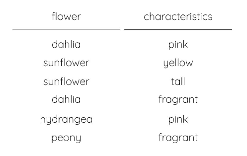
This format isn’t easily usable because of the duplicate rows with the same primary key. In the data structuring step, you would want to restructure the dataset so that each characteristic is its own column, making the data easier to use in the analysis. 

Data structuring examples

Let’s look at some examples of how you can restructure your data to better work for your data modeling and analysis downstream. It’s important to think about how you will be using this data so you can properly restructure it before the next step which is data cleaning. 

Unnesting a JSON object

If you come across a column that exists as a nested JSON object, you need to unpack this so that you will be able to use the values downstream. JSON is a format that can’t be natively used with standard SQL so it is required that you turn it into columns and values during the data structuring step. 

Luckily, most cloud data warehouses have functions built in for handling JSON objects. You can add these to your data models to unnest a JSON object and extract the keys and values. 

For example, Snowflake has two functions that can be used for unnesting JSON objects- PARSE_JSON() and TO_JSON(). 

PARSE_JSON() can be applied to a JSON object to produce a variant value. Then, after doing this, you can specify the key name in order to pull the value from the object. You will want to parse the values from each key in its own column. You can do this like so:

WITH parsing_json_object AS (

SELECT

    parse_json('{"name":"John", "age":30, "car":null}') AS json_object_to_parse

FROM car_dealership

) 

SELECT 

   json_object_to_parse: name AS name, 

  Json_object_to_parse:age AS age, 

  Json_object_to_parse:car AS car

FROM parsing_json_object 

Now, instead of a JSON object that you can’t apply SQL logic to, you instead have three separate columns, all of which you can use in your data model. 

AS for the TO_JSON() function, you can apply this to an object that has the same format as a JSON object, but may be a different column type. Applying this and then the PARSE_JSON() function will get you the same results as above. 

SELECT

    parse_json(to_json('{"name":"John", "age":30, "car":null}')) AS json_object_to_parse

FROM car_dealership

Here, you just need to change the data type before applying the same function as above. 

In Redshift, you can use the functions IS_VALID_JSON() and JSON_PARSE() for similar results. When reading JSON columns into Redshift, I like to begin with a simple CTE using one of these functions on the specified JSON column. In the next CTE, I read the specific columns from that JSON object and perform whatever cleanup I need to get the column value how I want. 

A staging model in dbt that reads from a source with a JSON column typically looks like this:

WITH 

orders_json_parsed AS (

SELECT 

  Order_id,

      Order_type,

  JSON_PARSE(order_details) AS order_details_json_parsed 

           FROM {{ source(‘application’, ‘orders’) }}

),

Orders AS (

SELECT

Order_id,

Order_type, 

Order_details_json_parsed.product_quantity AS order_product_quantity, 

Order_details_json_parsed.ship_date AS order_ship_date, 

Order_details_json_parsed.is_repeat_order AS is_repeat_order 

FROM orders_json_parsed

)

SELECT * FROM Orders

Most of the time dealing with JSON objects just requires knowing the right JSON functions to use with your data warehouse, and knowing how to extract those key-value pairs. 

Pivoting a table

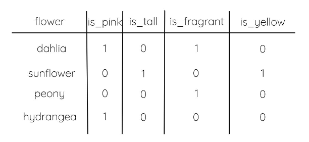
If you’re unfamiliar with pivot tables, they help to turn unique values in a column into their own column, filling in the corresponding cell for that row with a boolean value. This is what we want to use for the flower example I layed out above! Pivot tables are a great way to aggregate and calculate whether certain values exist in your data. For many cases, they can help you ensure you have a unique primary key across all of the columns in your data table. 

Here’s that flower example again:

Instead of all of the characteristics existing in one column, we want to create a few different columns- is_orange, is_fragrant, is_alive, and is_annual. These columns will be booleans and let us know whether a flower has that characteristic or not. 

If you’re a dbt user, then you know how easy the tool makes it to transform your data. While various SQL dialects have pivot and unpivot functions, dbt makes it easy by providing a pre-built function. It is dynamic, handling code changes for you and removing the complexity that comes with coding this logic otherwise.

For example, different data warehouses like Snowflake offer pivot functions to use with your SQL code. However, in order to make the functions dynamic, you need to layer code on top of the pivot function. This often requires writing some type of looping function or using a coding language other than SQL. 

Luckily, the pivot macro in the dbt_utils package pivots values from rows to columns. It is a dynamic piece of code, meaning you don’t have to specify the specific columns and rows in the table you are pivoting. It automatically finds them for you!

In order to pivot the characteristic column into separate columns, you need to specify it in the pivot function as well as in the dbt_utils.get_column_values function within the pivot function. Also, be sure to specify the name of your raw data source within the dbt_utils.get_column values function. This should match the source you are selecting from in your query!

select

  flower_name,

  {{ dbt_utils.pivot(

      'characteristic',

      dbt_utils.get_column_values(ref('flowers'), 'characteristic')

  ) }}

from {{ ref('flowers') }}

group by flower_name

For each flower name, this function will find the count of each characteristic and display that number in the characteristic’s column name. 

This macro also has a bunch of different arguments you can use to ensure you are getting exactly what you want from the function. Some of these include specifying the aggregate function you want to use and the column alias prefix/suffix for the resultant columns.

Not to mention, this package also has an unpivot macro if you need to perform the opposite result on your columns! 

Moving on to data cleaning

With data wrangling, you start with data discovery which helps you understand the data better so that you can properly clean it. You then move on to data structuring which makes it so you can actually clean the data in the next step. It helps make your data usable by putting it in the proper format.

Unnesting JSON objects and pivoting tables will ensure you have the columns and values you need to standardize your data in the next step of data wrangling. However, a lot of times with ETL tools, your data is already structured and you can skip this step entirely. 

In the section, we will discuss the most important step of data wrangling: data cleaning. This is where a lot of the magic happens. In my opinion, data cleaning makes up 70% of the data wrangling work! It’s also a step where data quality can be compromised if you don’t follow the correct precautions. 

Madison Schott is a modern data stack engineer for ConvertKit, an email marketing platform. She blogs about analytics engineering, data modeling, and data best practices on Medium. She also has her own weekly newsletter on Substack.