


SQL is the universal language of data modeling. While it is not what everyone uses, it is what most analytics engineers use. SQL is found all across the most popular modern data stack tools; ThoughtSpot’s SearchIQ query engine translates natural language query into complex SQL commands on the fly, dbt built the entire premise of their tool around SQL and Jinja. And within your Snowflake data platform, it’s used to query all your tables. SQL is used in every step from data ingestion to visualization.
However, just because you know how to write all the top SQL analytics functions and use them effectively within your stack, doesn’t mean you know the best practices when using it to write your data models. I’ve seen lots of data models that utilize various SQL functions and joins, but use them incorrectly. In the end, this results in suboptimal SQL queries, slowing down your data models and making them impossible to reuse in the future. Effective SQL query optimization is essential for improving the performance of your data models. By using SQL the right way, you can optimize your data models for readability, modularity, and performance- key indicators of a well-written data model.
In this article, I’ll discuss the top SQL data modeling mistakes I see and how you can fix them. These include using the wrong type of join, waiting until the end of the model to remove nulls and duplicates; using poorly named columns, aliases, and models; and writing overly-complicated code instead of a simple window function. Let’s dive in!
Mistake #1: Using the wrong type of join
There are different kinds of SQL joins that you’ll often see in data models. While left joins and inner joins are most common, I’ve also seen right joins and full outer joins. Remember, joins are used to merge two tables on a common field. Let’s review the differences between each of these.
LEFT JOINs select all of the data from the left (or first) table specified and the matching records from the right (or second) table specified in the join. So, if the value you are joining on is present in the second table but not the first, that row will not be included in the final output.
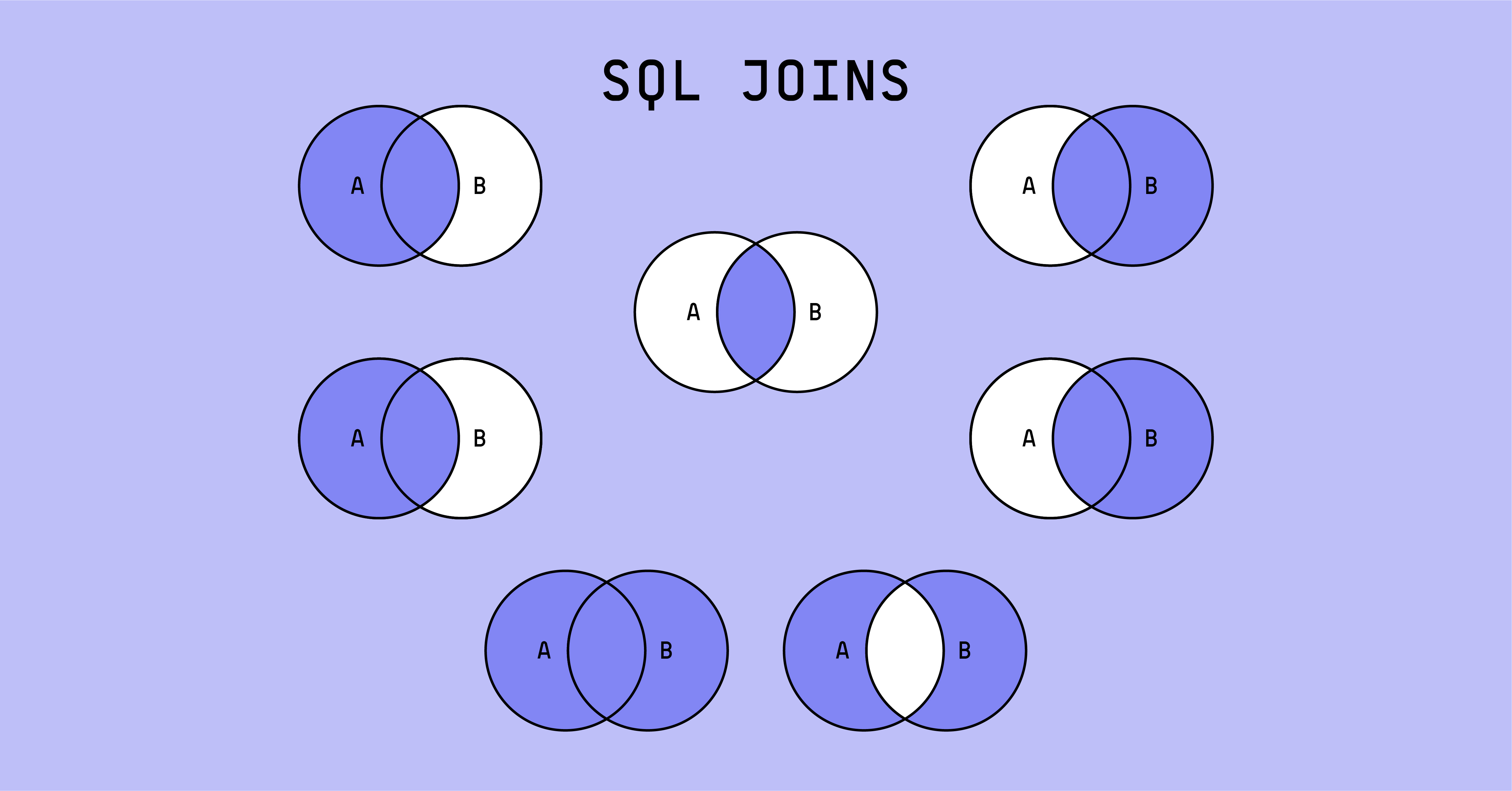
RIGHT JOINs are the exact opposite of LEFT JOINs. They select all of the data from the right (or second) table specified and the matching records from the left (or first) table specified in the join.
When modeling with SQL, you always want to use a LEFT JOIN over a RIGHT JOIN. If you’re using a RIGHT JOIN in your code, you’ll want to change the order you specify your tables to use a left join instead. It’s much easier for us to understand left joins compared to right. We often visualize from left to right, making it easier to comprehend which rows will and won’t be included in the resultant table. This will make your code more readable, a key pillar mentioned in the introduction.
Let’s say you have an initial query that looks like this:
SELECT
Customers.customer_name,
  Customers.customer_id,
  Address.street,
  Address.city,
  Address.state,
  address.zipcode
FROM address
RIGHT JOIN customers
ON customers.address_id = address.address_id
This can be hard to understand because of the way the tables are ordered with right joins. In this case, all the customer data will be present and only the addresses that match an address_id in the customers table will also be present. However, this isn’t very clear. Instead, you’d want to rewrite this to use a LEFT JOIN:
SELECT
  Customers.customer_name,
  Customers.customer_id,
  Address.street,
  Address.city,
  Address.state,
  address.zipcode
FROM customers
LEFT JOIN address
ON customers.address_id = address.address_id
Now, it is much easier to read and understand what the join is trying to do.
INNER JOINs select only records that are present in BOTH tables specified. So, if a record is in one table but not the other, that record will not be present in the final output.
INNER JOINs are great to use when you don’t want any null values in your resulting table. Because only rows present in both tables will be joined, you won’t have any null data columns, unlike with the other types of joins.
FULL OUTER JOINs select all records from both tables. Keep in mind that there will be a lot of null columns here for the records that are present in one table but not the other.
Mistake #2: Waiting until the end of the model to remove duplicate and null values
If you wait until the end of your data model to remove duplicates or null values, then you are slowing down the performance of your data models for no good reason. Removing duplicates and nulls at the very beginning of your data models will speed them up, helping you deliver data faster.
Replacing Nulls
SQL has a lot of helpful functions that you can use to replace null values at the very beginning of your data models. These can be particularly useful when bringing in data columns from your source tables.
COALESCE() takes in a list and returns the first non-null value. This is a good function to use to populate a column that could be made from a few potential columns. It’s a good idea to include a default string value as well in case all the columns specified are null.
SELECT
  Customer_name,
  COALESCE(home_phone, mobile_phone, email, ‘none’) AS preferred_contact
FROM customers
IFNULL() works similarly to COALESCE() but only takes in two values rather than a list. You first must specify a column and then a default value. This is a good function to use to replace null values in a column with a pre-determined default.
SELECT
  Customer_name,
  IFNULL(birthday, ‘01/01’) AS yearly_discount
FROM customers
ISNULL() returns 1 or 0 depending on whether the expression is null or not. It only takes in one expression unlike the other two functions which take in two or more values. This function most likely won’t be used as much as the others, since it is returning a boolean, but there are still cases where it could be helpful.
Filtering Nulls
Sometimes you may want to filter out rows that have null values for certain columns, rather than replacing those values. This is when a filtering function would work best.
The best way to filter for null values, or filter out null values, is by using a simple WHERE clause. You can specify the column you wish to search for nulls and whether you want your query to only include those nulls or include all rows without those nulls.
If we wanted to send an email to all users who have previously placed an order on our website, we could filter for WHERE order_id IS NOT NULL. This will give us only users who have previously ordered from the company.
SELECT
  User_id,
  Email
FROM  users
WHERE order_id IS NOT NULL
In contrast, if we wanted to send an email encouraging users with an account but no orders to place their first order with the company, we could find these users by running the following query:
SELECT
  User_id,
  Email
FROM  users
WHERE order_id IS NULL
When using these functions it’s important to keep your end goal in mind. Do you want rows with certain null values? Or do you want rows without nulls? This will determine which of these you wish to use.
Removing Duplicates
By leaving duplicates in your data model, you are computing calculations on rows that you are otherwise going to remove. In order to keep this from affecting performance, it’s best to remove duplicate rows early on. This way, your data models’ performance will be optimized from the very start.
There are two main ways to remove duplicates using SQL. In many cases performance for these two functions is equal, however, it does vary case by case. If you are trying to make your model as fast as possible, you can test both of these functions to see which is faster at removing duplicates in your scenario.
DISTINCT is the most common way to remove duplicates. This results in unique rows across the columns that you specify. You can apply this to your entire dataset by running SELECT DISTINCT * FROM dataset, or on a few columns that you wish to use in your model.
SELECT DISTINCT
  Name,
  Email,
  Phone
FROM customers
This query will only return rows that have a unique combination of the columns name, email, and phone.
GROUP BY column HAVING COUNT(*) > 1 is an example of a query you can use to find duplicate rows. While this one is a bit more complicated, it may be faster in certain cases. This function requires you to first GROUP BY the columns you want your rows to be unique across and then use the HAVING clause to check for the rows that exist more than one time.
Rather than removing duplicates, this function is better at identifying duplicate rows. You could also change the HAVING clause to specify COUNT(*) = 1 to only select rows that are not duplicates.
Using the same columns and dataset as the DUPLICATE example above, let’s see how this would look using this function.
SELECT
  Name,
  Email,
  Phone
FROM customers

GROUP BY name, email, phone
HAVING COUNT(*) > 1
This query specifically returns all of the rows that are duplicates, meaning more than one of these rows exist in your dataset.
Lastly, you can use the ROW_NUMBER() window function to assign a combination of column values to a number, and then filter these numbers for only a row number of one. We’ll get into window functions more in the next section.
Start Getting Better Insights
Mistake #3: Writing complex, long-running code that can easily be replaced by a window function
Many times, people will write extremely complex SQL code to solve a very specific problem when they could have used a window function. Window functions have the power to simplify extremely complex code so that it is both readable and performant. This is because fewer rows are typically examined and fewer temporary tables are created. They are often perfect for replacing subqueries, self-joins, and complex filters within queries.
Window functions work by using a PARTITION and ORDER BY clause. The PARTITION clause allows you to separate your calculations into groups. The ORDER BY clause then allows you to specify how you wish to order these groups. For example, with ROW_NUMBER(), you may want to PARTITION your data by each of the columns to find duplicate values. In this case, ORDER BY wouldn’t be necessary since you are looking for rows of the same values.
To eliminate duplicate rows using ROW_NUMBER(), you would specify the columns you are comparing and then create a column for row_number using the ROW_NUMBER() window function.
SELECT
  Order_id,
  Customer_name,
  Customer_state,
  ROW_NUMBER() OVER(PARTITION BY order_id, customer_name, customer_state) AS row_number
FROM recent_orders
Here, any rows that have duplicates will have row numbers other than 1. You can filter these duplicates out by then applying a filter where the row number is equal to 1.
SELECT
  Order_id,
  Customer_name,
  Customer_state
FROM recent_order_row_numbers
WHERE row_number = 1
Let’s say you now want to find a customer’s first order. You will need to use the ORDER BY clause to rank a customer’s order by the date that it was placed. For this, we can use a window function called RANK(). This works similarly to ROW_NUMBER() in that it assigns rows a number which you can then use to filter your queries. The only difference here is that RANK() will assign a row the same number if there is a tie in what it’s ordering by.
SELECT
  Order_id,
  Customer_id,
  Order_date,
  RANK() OVER(PARTITION BY customer_id ORDER BY order_date ASC) AS order_rank
FROM orders
RANK() assigns each row a number based on the order_date. Note how I added the ASC after the column to order by to tell the function which way to order the values. In this case, the order with the oldest date will have a rank of 1. You can also order a column by DESC values.
SELECT
  Order_id,
  Customer_id,
  Order_date
FROM ranked_orders
WHERE order_rank = 1
Now, by filtering on an order rank of 1, we are left with only a customer’s first order ever placed.
The last window function I want to mention is FIRST_VALUE(). This function finds the first value in an ordered list, replacing the need to filter by row number or rank. This function is great because it eliminates an extra step required with the other two functions. For the same example, you can run a query using FIRST_VALUE() instead of RANK() and get the output you’re looking for in one common table expression (CTE) rather than two.
SELECT
Customer_id,
  FIRST_VALUE(order_id) OVER(PARTITION BY customer_id ORDER BY order_date ASC) AS order_rank
FROM orders
Here, I can include the actual column name within the first part of the FIRST_VALUE() function to output the first order id ever placed by the customer. This eliminates the need to do any further filtering since the function is simply returning the value that I’m looking for.
Mistake #4: Using poorly named columns, aliases, and models
This is another mistake I often see that makes SQL data models extremely hard to read and understand. Often we want to finish coding a model as fast as possible to deliver on the end goal. By prioritizing speed, we neglect the code we are writing which only pushes problems further down the line. Just because it runs efficiently, doesn’t mean it’s well-written SQL code. Again, code needs to be readable, modular, and performant.
When writing SQL code, you need to use properly named columns, aliases, and models. When these aren’t intuitive to the reader, it makes code harder to understand when debugging or rewriting. Names should be clear and directly related to what they are describing.
Naming your data models
If you saw a reference to a data model named users_subs in SQL code, would you have any idea what type of data that model contains? We shouldn’t have to scour through code to find out what another data model is referencing. It should be explained within the model name itself. It’s a best practice to name a data model after the function it’s performing. For example, if you are joining two datasets named users and subscriptions, you should name your data model“users_joined_subscriptions”. Or, if your data model is calculating marketing spend for each platform, it should be called “marketing_spend_summed”.
Naming your columns
Column names should also be intuitive and describe exactly the data they contain. While naming here isn’t usually as big of a problem, column names tend to lack standardization. I’ve found that it’s common for columns to have different capitalization, verb tenses, and cases. This can create a lot of tech debt in your data models.
By following the same standards across all column names, you know what to expect when coding your SQL data models. A unified standard also helps communicate that the columns are safe to use and contain accurate data. I highly recommend creating some sort of style guide for how you name your columns. This should include things like what tense to use, how to specify a timezone, how to tell the difference between timestamp and date columns, and what capitalization to use.
For example, timestamp columns in my data models are always named as a past tense verb followed by an underscore and “at”. So, event_created_at or ordered_at would denote timestamp columns. My date columns are simply a noun followed by an underscore and “date”. Order_date or event_date would denote date columns. These standards are clear and make it easy to use these columns within models, already knowing their datatype.
Using descriptive aliases
Lastly, when using CTEs or tables within your SQL data models, it’s extremely important to use aliases that make sense to the reader. It is so common to use abbreviations for tables that are being joined or CTEs. However, these abbreviations often only make sense to the person that originally wrote the code. Take the extra time to spell out the entire table names or a CTE name that is descriptive of what the query does. The naming of CTEs should follow the same guidelines as the data modeling naming mentioned above.
Now let’s look at an example of a query that uses table aliases that are confusing and hard to read:
WITH
User_ subs AS (
  SELECT
    U.user_id,
    U.name,
    S.subscription_start_date
    S.subscription_end_date
  FROM users u
  LEFT JOIN s
  ON u.subscription_id = s.subscription_id
  WHERE s.subscription_status = ‘Cancelled’
),

Subscriptions AS (
  SELECT
    User_id,
    User_name,
    DATEDIFF(month, subscription_start_date, subscription_end_date) AS subscription_length
  FROM subscriptions
)

SELEC * FROM Subscriptions
It’s hard to understand which table these columns are coming from. This gets even more difficult as the queries grow in complexity. Instead of taking the easy way out, write out the full names to save future headaches. You also can’t understand what is happening in each CTE just by reading the name. You can guess it has something to do with users and subscriptions, but not the exact details. The above query should look like this:
WITH
users_joined_subscriptions AS (
  SELECT
    Users.user_id,
    Users.name,
    Subscriptions.subscription_start_date
    Subscriptions.subscription_end_date
  FROM users
  LEFT JOIN subscriptions
  ON users.subscription_id = subscriptions.subscription_id
  WHERE subscriptions.subscription_status = ‘Cancelled’
),

Subscription_length_calculated AS (
  SELECT
    User_id,
    User_name,
    DATEDIFF(month, subscription_start_date, subscription_end_date) AS subscription_length
  FROM users_joined_subscriptions
)

SELECT * FROM Subscription_length_calculated
See how much easier that is to understand? Now we can see which column comes from which table, without having to constantly reference which abbreviation is for which table. You can also understand exactly what’s happening in each CTE by just looking at the name.
Applying these SQL fixes to your data models
The key to writing high-quality SQL data models is writing SQL code with readability, modularity, and performance in mind. Assigning your assets descriptive names, using window functions, removing duplicate and null values at the beginning of your models, and using the right type of join will help you do this.
By correcting these four mistakes in your existing data models, you can prevent future tech debt within your data team as well as increase the reliability of your data pipeline. Keeping these mistakes in mind for future SQL data modeling will also help you write better quality code, ensuring your models will last a long time without having to be rebuilt.
If you’re ready to move beyond syntax errors and empower more business users to uncover powerful insights without writing a line of SQL, sign up for a free trial of ThoughtSpot today.
Madison Schott is an analytics engineer for Winc, a wine subscription company that makes all its own wines, where she rebuilt its entire modern data stack. She blogs about analytics engineering and data best practices on Medium. She also has her own weekly newsletter on Substack.


