

In the last article, we walked through a condensed history of computational language models that are the foundation for ChatGPT. We’ve managed to completely avoid talking about how various neural networks are wired and the math behind them. But now as we build toward the Transformer Architecture which is the workhorse for ChatGPT, we must indulge a bit into details to make sense of it. We will start with a few basic definitions, then cover the following topics:
Feed-forward networks
RNNs: Simplest neural networks that can deal with sequential data
LSTMs: A special class of RNNs that can have a longer short-term memory compared to vanilla RNNs
Transformer: The neural network architecture that made ChatGPT and other LLMs possible.
Machine Learning
Consider a function F that takes input vector X and outputs a vector Y.
F(X) = Y
Usually, most of the time in computing, we are given the function F and the input X, and we are supposed to compute Y. For example, F may be a linear function such as F(X) = 3X + 2 and given a value of X = 5, we compute Y = 3*5 + 2 =17.
In machine learning, we invert this paradigm, and given examples of inputs and outputs, we want to compute the function. For example, if we give you pairs of inputs (x=0, y=2), (x=1, y=5), (x=2, y=8), etc., you may guess that F is 3X + 2.
However, the relationship between X and Y is not that simple most of the time. You can only figure out F to a rough approximation. For example, given a set of points, you may be able to fit a straight line that goes close to these points. This is often called linear regression. In one dimension, linear regression can be described as F(X) = aX + b, and given a set of points, we need to find the best value of a and b. In this case, a and b are programmable parameters of a linear function.
You could also try and fit a quadratic function F(X) = aX2 + bX + c. Now there are three parameters to adjust so that the function fits the data. We could also fit an exponential curve F(X) = aXb with two parameters a and b. There can be many different families of functions to choose from and each family comes with its own set of parameters that can be picked to best fit the data.
In general machine learning is the process of choosing the right type of function and then finding the values for the parameters of that type of function that best fit the training data.
Neural Networks and Parameters
Artificial Neural Networks (ANN) are a class of parameterized mathematical functions inspired by the biological neurons in our brains. On average, a neuron in our brain is connected to roughly ten thousand other neurons. The neurons communicate through electrical impulses. The strength of connections between neurons determines how strong of an impulse gets communicated from one neuron to another. As we learn things or forget things, the strength of these connections changes. When the total strength of all the impulses arriving at a neuron exceeds a threshold, that neuron fires and sends an electrical impulse to downstream neurons.
Similarly, in an ANN, artificial neurons are connected to other artificial neurons and the strength of the connection between a pair of neurons is a programmable parameter that is set during the training process. Often neurons are organized in layers. The first layer is called the input layer and the last layer is called the output layer. Different layers are connected in a specific way which is determined by the architecture of the network chosen by its author. The more programmable connections the network has, roughly the more things it can learn or remember. A large number of programmable parameters or connections also means it takes more training data to train something meaningful and it takes more computing to train the network or to use.
Start Getting Better Insights
Feedforward networks
Things started with what we call feedforward networks. In this model, you have a sequence of neural network layers that sit on top of each other such that output from one layer feeds the input of the next layer so that when you provide the input at the first layer and run through the computations we get the output of the neural network. Each layer usually consists of a matrix of weights W that when multiplied to the input vector produces an output vector. From there, we can apply a non-linear function to each of the values of the output vector.
These kinds of networks represent a pure function that given the input can compute the output but not remember anything when the next input is provided. For example, you could train a feed-forward network to take all the pixel values of an 8x8 image and output 1 if it represents an image of a digit and zero otherwise.
They are great for processing fixed-size inputs to produce fixed-size outputs, but not great for processing a variable-sized sequence (for example a sequence of words of arbitrary length) and producing variable-sized output (for example, another sequence of words that represents the translation of words.)
Recurrent Neural Networks (RNNs)
Recur means to happen repeatedly or after an interval. In Recurrent Neural Networks (RNNs), the same calculation happens over and over again as you process time series data or a sequence of words of arbitrary length.
Let us consider a very simple problem, where you are given the number of times an API gets called every second. You want to alert if this number goes above thousand calls per second. But since the data is very noisy and you don’t want to alert unless there is a sustained large burst. So you choose to take an exponential average of the number of API calls per second and if that exponential average exceeds above thousand then you alert. Suppose xt describes the number of API calls at time t, ht denotes the exponential average with a decay of 0.9, and yt describes whether to alert or not. Then you could describe the calculation of yt as follows:
h0 = 0
hi = 0.9 hi - 1 + 0.1 xi
yi = 1 if hi > 1000 else 0
The second and third line of calculation re-occurs for every time step i. This is an example of how you process a variable-length sequence and output another variable-length sequence. Now let us generalize this idea to arbitrary vectors and arbitrary functions.
hi = F1(hi - 1, xi)
yi = F2(hi - 1, xi)
The only difference between the previous version and this version of the equation is that we have used arbitrary functions F1 and F2 instead of concrete functions for exponential averaging with a certain decay. In an RNN, F1 and F2 are feed-forward networks that are trained based on training data.
You can train RNNs to read a sequence of word embeddings and output its translation. You can also train an RNN to take historical weather data and forecast weather for the next day. Whenever input or output involved sequences, RNNs were the architecture of choice for a period of time.
What differentiates RNNs from feed-forward networks is the element of feedback. The output hi computed at step i is then fed back to the network at step i + 1. This feedback mechanism helps the network remember some information from the past. This feedback mechanism also makes training these networks harder. In particular, if the task required the network to remember something from multiple time steps away.
If you want to learn more here is a great resource.
Long Short-Term Memory (LSTM) Networks
LSTMs are a special class of recurrent networks that was designed to have a longer short-term memory of the recent past than basic RNNs.
Let us consider a problem similar to the above where we are given the number of times an API gets called every second, but now we want to alert if, for five consecutive seconds, there are zero API calls. This could mean an outage of some kind. Now we are no longer able to solve this by exponential averaging. One way to do this would be to maintain a sliding window for the last five values and alert whenever the total over that window is zero. Now the math looks like the following:
Window0 = {}
Windowi = Windowi -1.erase( xi - 5).insert(xi)
yi = 1 if sum(Windowi) = 0 else 0
Jumping from this to LSTM is a little more hand-wavy than before, but the same idea applies. If the function for what gets stored in the internal state (Window) and the Function for what gets forgotten from the internal state is computed using feed-forward neural networks, you have the concept of an LSTM.
The key reason this works better than basic RNNs is that it is able to remember more about the input from multiple previous steps. Its short-term memory stays longer. Both for RNNs and LSTMs, this is a great resource.
Attention
This was another very important idea that substantially advanced how state-of-the-art models behaved. Suppose you were translating the French sentence je suis étudiant to I am a student. The word je maps to I, the word étudiant maps to student. Suis sort of maps to both am and a. So if you wanted to see which word to pay attention to when producing the corresponding word, the following matrix would be very helpful.

In order to appreciate how this problem gets more complex, let's look at the picture below:
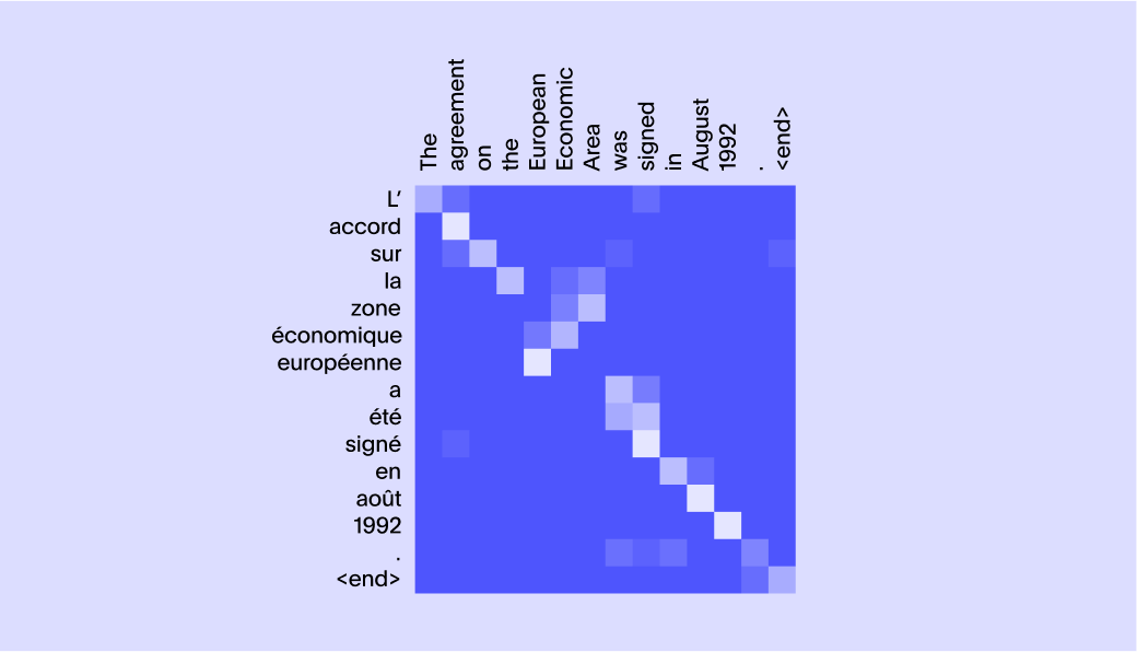
You will notice that some of the words need information from more than one word and it is certainly not a one-to-one mapping.
Interestingly, if the words are changed slightly the attention matrix also changes. For example, in the sentence “The lamp could not be packed into the suitcase because it was too large” the word “it” refers to the lamp. But in the sentence “The lamp could not be packed into the suitcase because it was too small.” The word “it” refers to the suitcase. So the only way to obtain these attention matrices would be to learn from data. This is exactly what was proposed in this breakthrough paper, Neural Machine Translation by Jointly Learning to Align and Translate.
One thing to note here is that when we’re talking about RNNs and LSTMs we are talking about arbitrary length sequences that could pass through these networks to produce a final vector. However, this approach was abandoned for two reasons. First, you cannot compute attention matrices unless the input and output length is capped to some limit. Second is the problem of vanishing gradients, which is a little harder to explain.
Most modern neural networks learn by propagating the error, or the difference between what the training label says the output should be versus what the current network is predicting. This means multiplying the partial derivative of every output with respect to the input for every node in the path from a given node to the output node. As the path length increases, there are higher and higher chances that this product of partial derivatives will grow either too large or too small. Too large means it will destabilize the training process and too small means training will not progress enough to achieve a good result. Both are bad.
For an RNN and LSTM, it was very hard to learn associations between words that are far apart. This led to an architecture where all the intermediate hidden states were passed on from encoder to decoder through the attention process. This again required that the network be limited to fixed-length sequences.
What is transformer architecture?
In 2017 researchers from Google published a new neural net architecture called transformer which has been the basis for most of the exponential progress in this field in the last four years. The paper was titled Attention is all you need because the central idea of this architecture is to rely on attention and self-attention instead of the feedback loop found in RNNs.
The transformer architecture is somewhat unique in its design compared to other architectures in that it is very hard to make sense of what is going on and why the authors are making certain choices. There are many details that you need to wrap your head around to make sense of it. However, there is solid intuition and reasoning behind the choices. In the following section, we’ll explore the key intuition behind this architecture.
The power of transformer architecture
There are two things that transformer architecture does very well. First, it does a really good job of learning how to apply context. For example, when processing a sentence, the meaning of a word or a phrase can completely change based on the context in which it is being used. Often how to apply this context is not just a function of grammar but a function of the relationship that exists in the real-world. Due to the self-attention mechanism in this architecture, it does a really good job of learning how to apply context in a data-driven way. Second, this architecture lends itself to much more parallelization of computing during training as well as inference. This allows for much faster throughput when learning from training examples and allows you to train larger networks with more training data at a given time scale. The largest transformer model with 213 million parameters in the original paper was trained over 3.5 days with 8 GPUs.
What is the self-attention in transformer models?
Self-attention is a mechanism for the network to contextualize words by paying attention to other words that make up its context in a body of text. The idea of self-attention is similar to the idea of attention introduced earlier, except that it’s used to contextualize words in a sentence as opposed to aligning words across translation as shown above.
Consider these two sentences:
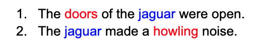
As you can see, the first sentence is talking about a car and the second is talking about the animal. How do we know? Because as humans we know that cars have doors and animals make howling noises. The only way to know this is to know a lot about real world concepts or objects and their relationship to each other.
To solve this problem, transformer models use neural networks to generate a vector called query, and a vector called key for each word. When the query from one word matches the key from another word, that means the second word has a relevant context for the first word. In order to provide appropriate context from the second word to the first word, a third vector called value is generated which is then combined with the first word to get a more contextualized meaning of the first word.
We are simplifying a lot of complex mathematics here, but one key thing to note is that for any such arrangement to work you need to design the math in a way that every function being used has a smooth slope (read: gradient) so that learning algorithms can find the optimal weights from examples. A lot of cleverness in transformers lies in designing these mechanisms so that the learning process converges and converges fast.
Another clever thing that the authors of transformers did was reduce the size of vectors for attention purposes, but have multiple parallel attention mechanisms going at once. This allows the neural network to have multiple shots at capturing different kinds of context. Also, having the self-attention layer repeat several times allows the network to combine context across larger phrases. For example, in the sentence “It was a knockoff of the 1984 ad from Apple.” First, you need to disambiguate the word “Apple” which in the context of an ad and 1984 is surely the company and not the fruit. Then you have the context to understand what 1984 means. Then you contextualize what “it” refers to. I am speculating here, but my guess is that this is where multiple layers of self-attention become very useful where you need to perform a chain of reasoning one after another.
In addition to self-attention, transformers also introduced the idea of positional encodings, making the network structure agnostic to the relative position of a word in the sequence.The position information is then added back as an input in the form of trigonometric functions. This was a very interesting choice and seems to have helped the efficacy of the network as well.
We are deliberately not going into the details of encoder layers, decoder layers, and other attention mechanisms in this article but if you’re curious to learn more I highly recommend reading The Illustrated Transformer.
Bidirectional Encoder Representations from Transformers (BERT)
Initially, transformer architecture didn’t grab much attention outside the machine learning community. But shortly after that, researchers at Google trained a new transformer model for NLP tasks that broke records on several fronts.
The model was trained to meet two objectives:
Guess missing words from a body of text
Given two sentences, guess if they were two consecutive sentences from a document two randomly chosen sentences from the entire training data.
In addition, the network was designed to output a vector embedding for the sentence so that it could be used for many different language tasks such as sentiment analysis, sentence similarity, and question answering using another small network on top of it.
What got everyone’s attention was that BERT was doing an amazing job on a number of language tasks and beating the state-of-the-art numbers. At this point it was not just a cool research idea. Various product teams in the industry including us started paying close attention to what was happening and figuring out a way to leverage the advances in this space.
The largest BERT model had 345 million parameters. It was trained on 64 tensor processing units (TPUs), a specialized learning hardware invented by Google, for four days at an estimated cost of $7,000. On one hand, it worried people that new innovation was taking more and more hardware investment but on the other hand, it clearly showed that larger models were smarter and able to capture a lot of knowledge. This caused two somewhat divergent camps: those who wanted to train larger and larger transformer networks for NLP to see how smart they get, and those that wanted to train smaller networks while preserving some of the goodness of BERT.
Generative pretrained transformer (GPT) vs BERT
Generative pretrained transformers are a family of Transformer models trained by OpenAI for Language Modeling tasks. The first GPT model pre-dates the BERT model. While BERT relied on clever training objectives, OpenAI went in the direction of training models to predict the next word (Language Modeling). The first GPT model had 117 million parameters and substantially moved state-of-the-art numbers for many tasks. But it wasn’t until GPT-2 with its 1.5 billion parameters that it started capturing public attention.
The initial idea behind GPT was to pre-train a network on language modeling tasks over a large body of text and then fine tune the network for various language tasks. In this way, you’d get to train on the model unsupervised, without any human-generated labeled data, but still take advantage of supervised training over smaller labeled data for specific tasks. Hence the term pre-training. However, what was even more surprising was that the task of language modeling itself became an extremely powerful tool. You could simply talk to the model and ask it to perform a task and it would surprise you with a somewhat intelligent answer.
The network was only trained to predict the next words given an input text, but depending on what text you supplied, the model showed signs of intelligence that would have been inconceivable just a few years ago. As a result, we started calling the input text a prompt. In the next article, you will see several examples of prompt text and GPT-3 responses, illustrating the emergent properties of large language models.
n fact, not just GPT, but multiple other LLMs have shown that once the model exceeds a certain threshold size (somewhere between 50 billion and 100 billion parameters), it starts demonstrating very interesting properties in terms of its ability to answer questions. In the next article, we’ll talk about the emergent properties of LLMs and how ChatGPT was trained further to take advantage of these capabilities.
ThoughtSpot brings this same shift to data analytics. With natural language search and AI-driven insights, ThoughtSpot lets teams interact with their business data just as intuitively. Ask a question, get a clear answer, and make confident decisions faster. Just like prompt-based AI changed the way we use language, ThoughtSpot is changing the way we use data.
Want to see this for yourself? Schedule a demo today.


